Page Not Found
Page not found. Your pixels are in another canvas.
A list of all the posts and pages found on the site. For you robots out there is an XML version available for digesting as well.
Page not found. Your pixels are in another canvas.
About me
This is a page not in th emain menu
Published:
Published:
Published:
Recall of the definition of conditional probabilities and chain rule \(P(A,B) = P(A|B) P(B)\) \(P(x_1,x_2,x_3,...,x_n) = P(x_1)P(x_2|x_1)P(x_3|x_1,x_2)...P(x_n|x_1,...,x_{n-1})\)
We do everything in log probs:
[(p_1 * p_2 * p_3 * p_4) <> \log p_1 + \log p_2 + \log p_3 + \log p_4]
[PP(W) = P(w_1w_2…w_n)^{1/N}]
| N-gram order | Unigram | Bigram | Trigram |
|---|---|---|---|
| Perplexity | 963 | 170 | 109 |
Published:
Imagine trying to devour a whole cake in one bite. It’s not only impractical but also overwhelming.
Human cognitive abilities have limits. When faced with a massive wall of text, our brains struggle to process and retain information effectively. By breaking down the text into manageable chunks we can mimic the natural way humans consume information, reducing cognitive load and enhancing comprehension.
Text chunking facilitates better contextual understanding. Instead of treating the entire document as a single entity, breaking it into smaller chunks enables us capture nuances and relationships within specific segments of the text.
Published:
Published:
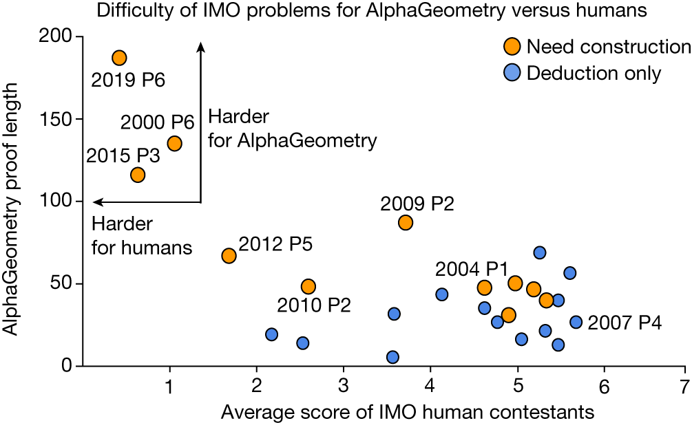
AlphaGeometry is an AI system developed by DeepMind that can solve complex geometry problems. It uses a combination of a neural language model and a symbolic deduction engine to solve problems. It was able to solve 25 out of 30 Olympiad geometry problems, which is between the average score of human silver and gold medalists.
The system was able to achieve this by generating a large amount of synthetic training data. This data consisted of millions of geometry problems and their solutions. AlphaGeometry was then trained on this data, and it was able to learn to solve new problems by analogy.
AlphaGeometry is a significant advance in the field of artificial intelligence. It shows that AI systems can now be used to solve complex problems that were previously thought to be the exclusive domain of humans.
Here are some of the key takeaways from the paper:
AlphaGeometry is a system that can solve geometry problems without any human demonstrations. It does this by using a combination of a symbolic solver and a large language model akin to the idea of thinking, fast and slow, one system provides fast, “intuitive” ideas, and the other, more deliberate, rational decision-making.
Because language models excel at identifying general patterns and relationships in data, they can quickly predict potentially useful constructs, but often lack the ability to reason rigorously or explain their decisions
Symbolic deduction engines, on the other hand, are based on formal logic and use clear rules to arrive at conclusions. The symbolic solver can reason about the things that already exist in the problem, but it cannot introduce new things. The language model is used to suggest new things to construct, such as points, lines, or circles.
AlphaGeometry was trained on a dataset of 100 million synthetic data examples.
Humans can learn geometry using a pen and paper, examining diagrams and using existing knowledge to uncover new, more sophisticated geometric properties and relationships. Our synthetic data generation approach emulates this knowledge-building process at scale, allowing us to train AlphaGeometry from scratch, without any human demonstrations.
The system starts by generating one billion random diagrams of geometric objects and exhaustively derived all the relationships between the points and lines in each diagram. Then it finds all the proofs contained in each diagram, then works backwards to find out what additional constructs, if any, were needed to arrive at those proofs. We call this process symbolic deduction and traceback.
The system works by first trying to solve the problem with the things that are already there. If it can’t solve the problem, it asks the language model for a suggestion. It then adds the suggestion to the problem and tries to solve it again. This process repeats until the problem is solved.
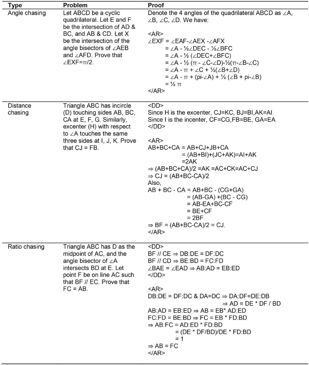
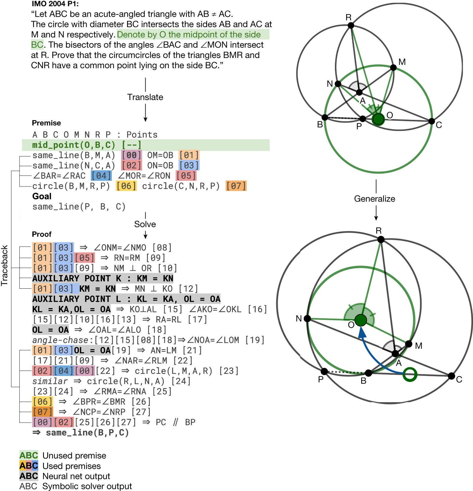
AlphaGeometry’s solutions have machine-verifiable structure. Yet despite this, its output is still human-readable.
One could have imagined a computer program that solved geometry problems by brute-force coordinate systems: think pages and pages of tedious algebra calculation. AlphaGeometry is not that. It uses classical geometry rules with angles and similar triangles just as students do.”
AlphaGeometry is a very specialized system that only works for a certain type of geometry problem. However, it is very good at solving these problems, and it is often better than humans.
Ablations and Main results 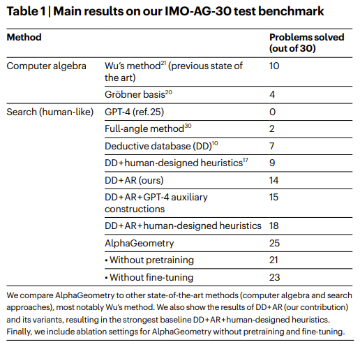
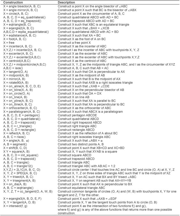
These actions include constructions to create new points that are related to others in a certain way, that is, collinear, incentre/excentre etc., as well as constructions that take a number as its parameter, for example, “construct point X such that given a number α, ∠ABX = α”.
One can extend this list with more sophisticated actions to describe a more expressive set of geometric scenarios, improving both the synthetic data diversity and the test-set coverage
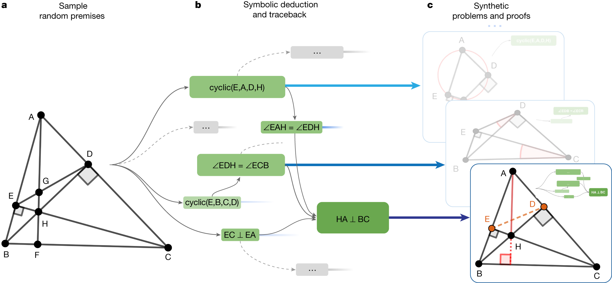
In the bottom example, points E and D took part in the proof despite being irrelevant to the construction of HA and BC; therefore, they are learned by the language model as auxiliary constructions.
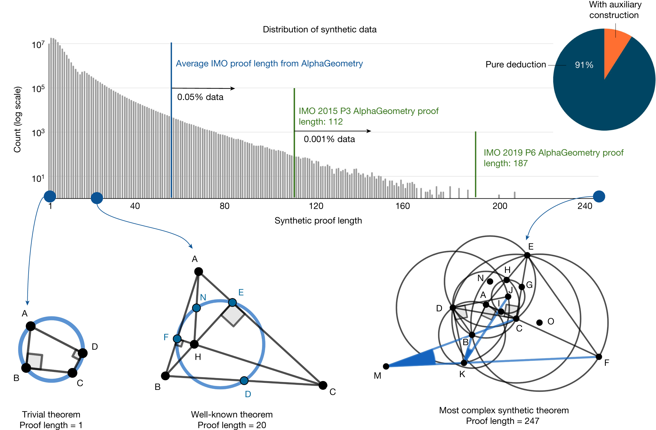
Of the generated synthetic proofs, 9% are with auxiliary constructions. Only roughly 0.05% of the synthetic training proofs are longer than the average AlphaGeometry proof for the test-set problems.
The most complex synthetic proof has an impressive length of 247 with two auxiliary constructions. Most synthetic theorem premises tend not to be symmetrical like human-discovered theorems, as they are not biased towards any aesthetic standard.
Focus on auxiliary constructions: The LLM is specifically trained to suggest new constructions that can be used to prove the problem. This is a key challenge in geometry problem solving, as it is often necessary to introduce new points, lines, or circles in order to prove a theorem.
Interpretable proofs: The proofs generated by the system are written in a natural language that is easy for humans to understand. This is important for debugging and verifying the proofs.
AlphaGeometry can only solve problems that can be expressed in its limited - language. Additionally, AlphaGeometry is not always able to find the shortest or most elegant proof.
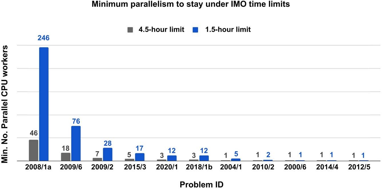
The minimum number of parallel CPU workers to solve all 25 problems and stay under the time limit, given four parallel copies of the GPU V100-accelerated language mode
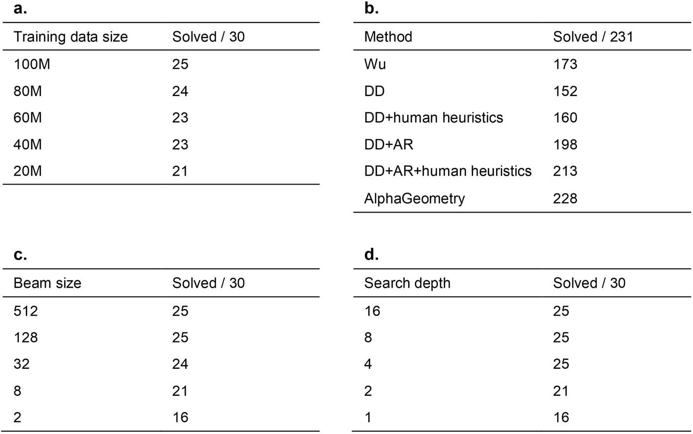
a, The effect of reducing training data on AlphaGeometry performance. At 20% of training data, AlphaGeometry still solves 21 problems, outperforming all other baselines. b, Evaluation on a larger set of 231 geometry problems, covering a diverse range of sources outside IMO competitions. The rankings of different machine solvers stays the same as in Table 1, with AlphaGeometry solving almost all problems. c, The effect of reducing beam size during test time on AlphaGeometry performance. At beam size 8, that is, a 64 times reduction from its full setting, AlphaGeometry still solves 21 problems, outperforming all other baselines. d, The effect of reducing search depth on AlphaGeometry performance. At depth 2, AlphaGeometry still solves 21 problems, outperforming all other baselines.
Neural Network Component: Typically a deep neural network (DNN) trained on large datasets. Extracts relevant features and patterns from input data. Represents knowledge in a continuous, distributed manner.
Published:
As we discussed in previous posts, the ability to properly formulate a Markov Decision Process (MDP) is imperative for successful application of Reinforcement Learning (RL) methods.
MDPs serve as a framework to formalize sequential decision-making problems, in which decisions over time are decomposed into a series of subproblems.
In canonical form, an MDP is described by a tuple $(S,A,R,P,\gamma)$.
By definition, any MDP fulfills the Markov property, aka the memoryless property. This property states that decisions do not depend on states of the past, but only on the present state. If the problem can be formulated in such a way, we can break down extremely complicated decision problems into a sequence of more manageable subproblems, to be solved independently.
It is natural to interpret the Markov property as ‘not utilizing any information from the past’. However, there is a distinction between not using states from the past and information from the past.
In mathematical terms, states including historical information are utilized in higher-order MDPs. Such models provide a richer representation of the system than first-order MDPs allow (which indeed only include present information). Taken to the extreme, a state could even include all historical information.
A state $s \in S$ contains all information needed to compute decisions, rewards, and transitions; the state space S is the set containing all states.
A core notion of MDPs is that decisions are made solely based on the current state of the system (the memoryless property); past states should not factor into decision-making. A common misunderstanding is that a state cannot incorporate past information; this is in fact allowed (higher-order Markov models, see Salnikov et al.).
In some cases a state is a simple scalar, such as an agent’s position on a one-dimensional line. Typically, the state would be a vector. Consider a robot arm, with the state described by the angles of its three joints $s=[x,y,z]$
A stock portfolio state may be described with the prevailing price level and amount held per stock $s=[p_1,p_2,…,p_n,s_1,s_2,…,s_n]$
As a guideline, the state should include exactly all relevant data used to make informed decisions — no less, no more. If certain data does not impact decision-making, rewards or transitions, it should not be incorporated in the state.
Wikipedia (n.d.) — “A state variable is one of the set of variables that are used to describe the mathematical ‘state’ of a dynamical system”.
Bellman (1957) — “… we have a physical system characterized at any stage by a small set of parameters, the state variables. ”
Puterman (2014) — “At each decision epoch, the system occupies a state.”
Sutton & Barto (2018) — “…signal to represent the basis on which the choices are made (the states)”
Bertsekas (2018) — “…is the state of the system, an element of some space. […] Many classical problems in control theory involve a state that belongs to a Euclidean space, i.e., the space of n-dimensional vectors of real variables, where n is some positive integer.”
Powell distinguishes three state components:
(i) physical: directly observable properties of the system, e.g., resources. Think the location of a truck, money on your bank account, or battery level of a drone.
(ii) information: non-tangible deterministic information. Can be directly observed, but is not necessarily a physical component of the system.
Aside from properties directly derived from the system, we often use additional information in decision-making. If we have a stock portfolio, the stock prices (market data) would be information.
Information can also pertain to the past or future. Past stock prices might reveal relevant trends that cannot be gleaned solely from the present price
(iii) belief / knowledge: non-tangible probabilistic knowledge. Concretely, the belief may be represented by the parameters of a distribution.
We might not make decisions based solely on known information, but also on uncertain information or beliefs.
Published:
The ability to properly formulate a Markov Decision Process (MDP) is imperative for successful application of Reinforcement Learning (RL) methods.
MDPs serve as a framework to formalize sequential decision-making problems, in which decisions over time are decomposed into a series of subproblems.
In canonical form, an MDP is described by a tuple $(S,A,R,P,\gamma)$.
By definition, any MDP fulfills the Markov property, aka the memoryless property. This property states that decisions do not depend on states of the past, but only on the present state. If the problem can be formulated in such a way, we can break down extremely complicated decision problems into a sequence of more manageable subproblems, to be solved independently.
It is natural to interpret the Markov property as ‘not utilizing any information from the past’. However, there is a distinction between not using states from the past and information from the past.
In mathematical terms, states including historical information are utilized in higher-order MDPs. Such models provide a richer representation of the system than first-order MDPs allow (which indeed only include present information). Taken to the extreme, a state could even include all historical information.
A state $s \in S$ contains all information needed to compute decisions, rewards, and transitions; the state space S is the set containing all states.
A core notion of MDPs is that decisions are made solely based on the current state of the system (the memoryless property); past states should not factor into decision-making. A common misunderstanding is that a state cannot incorporate past information; this is in fact allowed (higher-order Markov models, see Salnikov et al.).
In some cases a state is a simple scalar, such as an agent’s position on a one-dimensional line. Typically, the state would be a vector. Consider a robot arm, with the state described by the angles of its three joints $s=[x,y,z]$
A stock portfolio state may be described with the prevailing price level and amount held per stock $s=[p_1,p_2,…,p_n,s_1,s_2,…,s_n]$
As a guideline, the state should include exactly all relevant data used to make informed decisions — no less, no more. If certain data does not impact decision-making, rewards or transitions, it should not be incorporated in the state.
Wikipedia (n.d.) — “A state variable is one of the set of variables that are used to describe the mathematical ‘state’ of a dynamical system”.
Bellman (1957) — “… we have a physical system characterized at any stage by a small set of parameters, the state variables. ”
Puterman (2014) — “At each decision epoch, the system occupies a state.”
Sutton & Barto (2018) — “…signal to represent the basis on which the choices are made (the states)”
Bertsekas (2018) — “…is the state of the system, an element of some space. […] Many classical problems in control theory involve a state that belongs to a Euclidean space, i.e., the space of n-dimensional vectors of real variables, where n is some positive integer.”
Powell distinguishes three state components:
(i) physical: directly observable properties of the system, e.g., resources. Think the location of a truck, money on your bank account, or battery level of a drone.
(ii) information: non-tangible deterministic information. Can be directly observed, but is not necessarily a physical component of the system.
Aside from properties directly derived from the system, we often use additional information in decision-making. If we have a stock portfolio, the stock prices (market data) would be information.
Information can also pertain to the past or future. Past stock prices might reveal relevant trends that cannot be gleaned solely from the present price
(iii) belief / knowledge: non-tangible probabilistic knowledge. Concretely, the belief may be represented by the parameters of a distribution.
We might not make decisions based solely on known information, but also on uncertain information or beliefs.
Published:
Published:
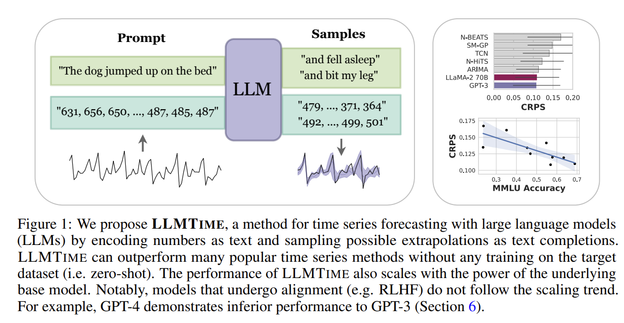
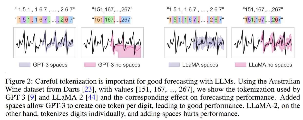
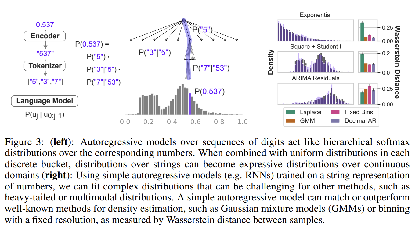
LLMs can assign likelihoods to full sequences of time series data, and we show how a small modification to an LLM’s discrete likelihood can yield a continuous density that is useful for model comparison
[0.123, 1.23, 12.3, 123.0 → “ 1 2 , 1 2 3 , 1 2 3 0 , 1 2 3 0 0”]
Rescaling $\alpha$-percentile to allow (1-$\alpha$) values to be seen by the LLM and give it the possibility of generating values higher than it has seen. Offset $\beta$. Hyperparameters tunned on validation log likelihood.
Sampling/Forecasting To forecast, draw many samples (e.g. 20) from the LLM and use the statistics of the samples at each time step to construct a point estimate (e.g. as the median) or probabilistic forecast (e.g. as quantiles). To control sampling, we use temperature scaling, logit bias, and nucleus sampling
LLMTIME with base model GPT-3 or LLaMA-2 70B has the best or second best aggregated performance on several deterministic time series benchmarks while being entirely zero-shot.
For some of the longer time series, not all of the history can be fit into the context window, and hence hyperparameters implicitly capture the trade-off between higher precision and capturing a larger temporal history
Deterministic Results 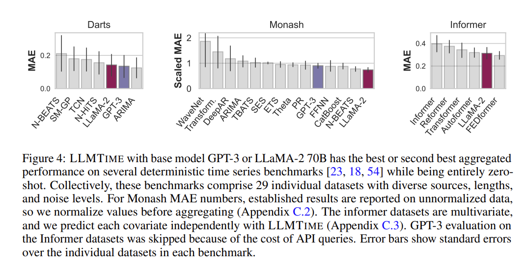

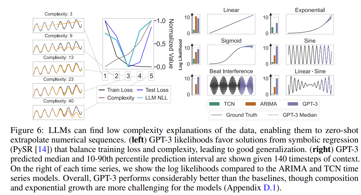
To understand why LLMs can extrapolate time series in a zero-shot manner, let’s take a step back and consider simple numerical sequences, for example $[1, 4, 9, 16, . . . ]$ or $[0, 0, 1, 0, 1, 2, 0, 1, 2, 3, . . . ]$.
For any input sequence, there are arbitrarily many generation rules that are consistent with the input (e.g. $f(x) = x^2$ for $x \in [1, 2, 3, 4, …]$), but some generation rules are overly complex and will generalize poorly
LLMs can forecast effectively because they prefer completions derived from simple rules, adopting a form of Occam’s razor prior.
To explicitly demonstrate this phenomenon, we create a synthetic example using the function $f(x) = x + cos(x)$ with additive Gaussian noise. We fit symbolic expressions to the first 70% of timesteps using PySR with symbols [”+”, “·”, “-“, “/”, “sin”, “cos”, “exp”,”square”] to identify generating rules with known complexity, quantified by the number of symbols in the regressed expression. The figure bellow shows that GPT-3 assigns the highest likelihood to symbolic regression generating rules that balance consistency with complexity.
LLMs can leverage their abilities in order to seamlessly incorporate missing data or answer questions about time series
Figure 7 (right) shows that chat versions tend to have markedly worse forecasting error than their non-chat counterparts, though still maintain trends in size and reasoning ability. 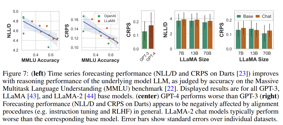
While the likelihoods of traditional methods rapidly deteriorate with corruptions, we find that LLaMA-2 70B is more resilient, and when comparing CRPS values, LLaMA-2 70B is competitive with methods that use interpolation.
Because LLMs are designed for natural language and code, we can augment the numerical time series with useful text. We can do so either by providing textual side information as inputs, or by producing textual outputs from a given time series.
An interesting question is whether GPT-4 can explain in text its understanding of a given time series, we probe this quality by providing GPT-4 the code to generate our synthetic time series, provide the values of one these time series, and then ask it to infer which of the functions produced the data in a zero-shot manner. The prediction accuracies are shown in Figure 8 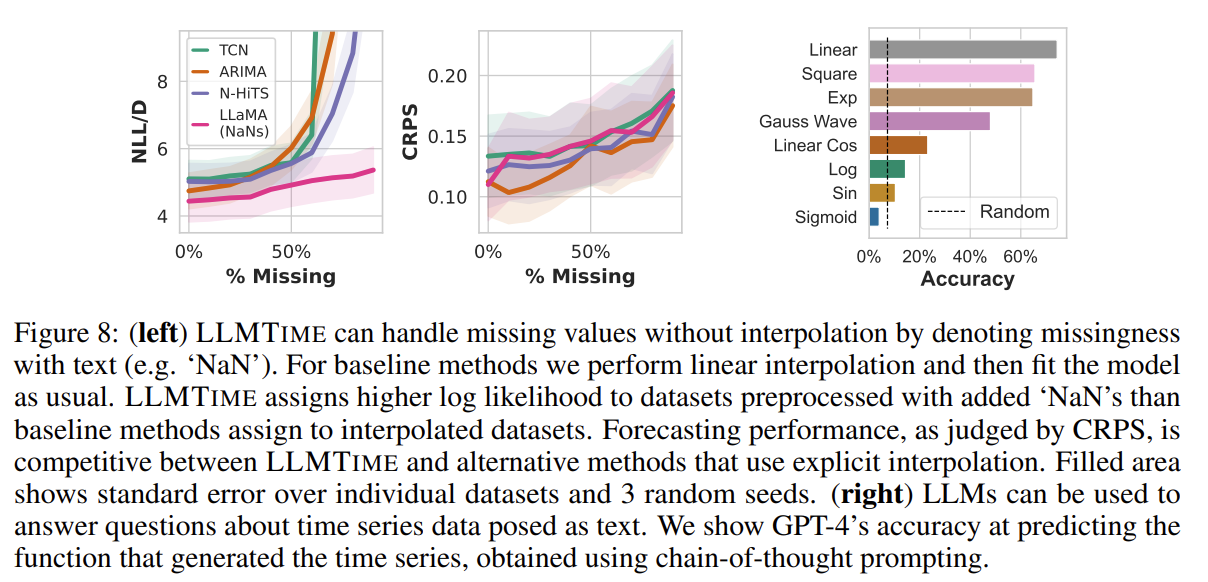
With CoT [47] prompting the model performs much better than random chance; however, its ability to identify patterns better when directly extrapolating the numerical data, suggesting that its numerical understanding is not fully connected to its textual understanding.
Published:
[CME.CL] active
[CME.HO]
Published:
Published:
Published:
Most of the quantitative finance measures build on the Markowitz’ mean-variance paradigm, which assumes that the mean and standard deviation of the distribution of one-period return are sufficient statistics for evaluating the prospects of an investment portfolio.
The historic Sharpe Ratio is closely realted to the t-statistic for measuring the statistical significance of the mean differential return. The t-statisic will equal the Sharpe Ratio times the square root of T (the number of returns used for the calculations). If historic Sharpe Ratios for a set of funds are computed using the same number of observations, the Sharpe Ratios will thus be proportinal to the t-statistics of the means.
The sharpe Ratio is not independent of the time period over which it is measured. This is true for both ex ante and ex post measures.
\(\sigma_d_T = \sqrt(T) \sigma_d_1\) \(S_T = \sqrt(T) S_1\)
In practice, the situation is likely to be more complex. Multiperiod returns are usually computed taking compounding into account, which makes the relationship more complicated. Moreover, underlying differential returns may be serially correlated. Even if the underlying process does not involve serial correlation, a specific ex post sample may.
It is common practice to “annualize” data that apply to periods other than one year. Doing so before computing a Sharpe Ratio can provide at least reasonably meaningful comparisons among strategies, even if predictions are intially stated in terms of different measurement periods.
To maximize information content, it is usually desriable to measure risks and returns using fairly short (e.g. montly periods). For purposes of standardization it is then desirable to annualize the results.
For example, an investment in a broad stock market index, financed by borrowing. Typical estimates of the annual excess return on the stock market in a developed country might include a mean of 6% per year and a standard deviation of 15%. The resulting excess return Sharpe ratio of the “stock market”, stated in annual terms would then be 0.40.
It is essential that the Sharpe Ratio is computed using the mean and standard deviation of a differential return (or more broadly, the return on what will be termed a zero investment strategy). Otherwise it loses its raison d’etre. Clearly, the Sharpe Ration can be considered a special case of the more general construct of the ratio of the mean of any distribution to its standard deviation.
Published:
Published:
We are now ready to summarize the four conditions that comprise “the simple linear regression model:”
Linear Function: The mean of the response, $\mbox{E}(Y_i)$ at each value of the predictor $x_i$ is a Linear function of the $x_i$.
Independent: The errors, $\epsilon_{i}$, are Independent. Normally Distributed: The errors, $\epsilon_{i}$, at each value of the predictor, $x_i$, are Normally distributed. Equal variances (denoted $\sigma^{2}$): The errors, $\epsilon_{i}$, at each value of the predictor, $x_i$, have Equal variances.
An equivalent way to think of the first (linearity) condition is that the mean of the error, $\mbox{E}(\epsilon_i)$, at each value of the predictor, $x_i$, is zero. An alternative way to describe all four assumptions is that the errors, $\epsilon_{i}$, are independent normal random variables with mean zero and constant variance, $\sigma^{2}$.
Maximum Likelihood Estimation (MLE) is a method used in statistics to estimate the parameters of a statistical model. The idea behind MLE is to find the parameter values that maximize the likelihood function, which measures how well the model explains the observed data.
The likelihood function, denoted as $L(\theta;x)$, represents the probability of observing the given data $𝑥$, given a set of parameters $𝜃$ for a statistical model. Mathematically, the likelihood function is defined as:
| $$L(\theta;x) = f(x | \theta)$$ |
| where $f(x | \theta)$ is the pdf or pmf of the data given the parameters. |
[\hat{\theta} = \arg\max_{\theta} L(\theta; x)]
[L(\mu; x) = \prod_{i=1}^{n} \frac{1}{\sqrt{2\pi\sigma^2}} \exp\left(-\frac{(x_i - \mu)^2}{2\sigma^2}\right)]
In general, degrees of freedom refer to the number of independent pieces of information that are available to estimate a parameter or calculate a statistic. The concept is often used to describe the number of values in the final calculation of a statistic that are free to vary without violating any constraints.
Consistency: Under certain regularity conditions, the MLE estimators are consistent, which means that as the sample size increases, the estimates converge to the true parameter values.
Asymptotic Normality: For large samples, the MLE estimators are approximately normally distributed, which allows for the construction of confidence intervals and hypothesis tests.
Efficiency: Among all unbiased estimators, the MLE provides the minimum variance, making it efficient.
Published:
Published:
Published:
Published:
The AI revolution drove frenzied investment in both private and public companies and captured the public’s imagination in 2023. Transformational consumer products like ChatGPT are powered by Large Language Models (LLMs) that excel at modeling sequences of tokens that represent words or parts of words [2]. Amazingly, structural understanding emerges from learning next-token prediction, and agents are able to complete tasks such as translation, question answering and generating human-like prose from simple user prompts.
Not surprisingly, quantitative traders have asked: can we turn these models into the next price or trade prediction [1,9,10]? That is, rather than modeling sequences of words, can we model sequences of prices or trades. This turns out to be an interesting line of inquiry that reveals much about both generative AI and financial time series modeling. Be warned this will get wonky.
LLMs are known as autoregressive learners – those using previous tokens or elements in a sequence to predict the next element or token. In quantitative trading, for example in strategies like statistical arbitrage in stocks, most research is concerned with identifying autoregressive structure. That means finding sequences of news or orders or fundamental changes that best predict future prices.
Where things break down is in the quantity and information content of available data to train the models. At the 2023 NeurIPS conference, Hudson River Trading, a high frequency trading firm, presented a comparison of the number of input tokens used to train GPT-3 with the amount of trainable tokens available in the stock market data per year HRT estimated that, with 3,000 tradable stocks, 10 data points per stock per day, 252 trading days per year, and 23400 seconds in a trading day, there are 177 billion stock market tokens per year available as market data. GPT-3 was trained on 500 billion tokens, so not far off [6].
But, in the trading context the tokens will be prices or returns or trades rather than syllables or words; the former is much more difficult to predict. Language has an underlying linguistic structure (e.g., grammar) [7]. It’s not hard to imagine a human predicting the next word in a sentence, however that same human would find it extremely challenging to predict the next return given a sequence of previous trades, hence the lack of billionaire day traders. The challenge is that there are very smart people competing away any signal in the market, making it almost efficient (“efficiently inefficient”, in the words of economist Lasse Pedersen) and hence unpredictable. No adversary actively tries to make sentences more difficult to predict — if anything, authors usually seek to make their sentences easy to understand and hence more predictable.
Looked at from another angle, there is much more noise than signal in financial data. Individuals and institutions are trading for reasons that might not be rational or tied to any fundamental change in a business. The GameStop episode in 2021 is one such example. Financial time series are also constantly changing with new fundamental information, regulatory changes, and occasional large macroeconomic shifts such as currency devaluations. Language evolves at a much slower pace and over longer time horizons.
On the other hand, there are reasons to believe that ideas from AI will work well in financial markets. One emerging area of AI research with promising applications to finance is multimodal learning [5], which aims to use different modalities of data, for example both images and textual inputs to build a unified model. With OpenAI’s DALL-E 2 model, a user can enter text and the model will generate an image. In finance, multi-modal efforts could be useful to combine information classical sources such as technical time series data (prices, trades, volumes, etc.) with alternative data in different modes like sentiment or graphical interactions on twitter, natural language news articles and corporate reports, or the satellite images of shipping activity in a commodity centric port. Here, leveraging multi-modal AI, one could potentially incorporate all these types of non-price information to predict well.
Another strategy called ‘residualization’ holds prominence in both finance and AI, though it assumes different roles in the two domains. In finance, structural `factor’ models break down the contemporaneous observations of returns across different assets into a shared component (the market return, or more generally returns of common, market-wide factors) and an idiosyncratic component unique to each underlying asset. Market and factor returns are difficult to predict and create interdependence, so it is often helpful to remove the common element when making predictions at the individual asset level and to maximize the number of independent observations in the data.
In residual network architectures such as transformers, there’s a similar idea that we want to learn a function h(X) of an input X, but it might be easier to learn the residual of h(X) to the identity map, i.e., h(X) – X. Here, if the function h(X) is close to identity, its residual will be close to zero, and hence there will be less to learn and learning can be done more efficiently. In both cases the goal is to exploit structure to refine predictions: in the finance case, the idea is to focus on predicting innovations beyond what is implied by the overall market, for residual networks the focus is on predicting innovations to the identity map.
A key ingredient for the impressive performance of LLMs work is their ability to discern affinities or strengths between tokens over long horizons known as context windows. In financial markets, the ability to focus attention across long horizons enables analysis of multi-scale phenomena, with some aspects of market changes explained across very different time horizons. For example, at one extreme, fundamental information (e.g., earnings) may be incorporated into prices over months, technical phenomena (e.g., momentum) might be realized over days, and, at the other extreme, microstructure phenomena (e.g., order book imbalance) might have a time horizon of seconds to minutes.
Capturing all of these phenomena involves analysis of multiple time horizons across the context window. However, in finance, prediction over multiple future time horizons is also important. For example, a quantitative system may seek to trade to profit from multiple different anomalies that are realized over multiple time horizons (e.g., simultaneously betting on a microstructure event and an earnings event). This requires predicting not just the next period return of the stock, but the entire term structure or trajectory of expected returns, while current transformer-style predictive models only look one period in the future.
Another financial market application of LLMs might be synthetic data creation [4,8]. This could take a few directions. Simulated stock price trajectories can be generated that mimic characteristics observed in the market and can be extremely beneficial given that financial market data is scarce relative to other sources as highlighted above in the number of tokens available. Artificial data could open the door for meta-learning techniques which have successfully been applied, for example, in robotics. In the robotic setting controllers are first trained using cheap but not necessarily accurate physics simulators, before being better calibrated using expensive real world experiments with robots. In finance the simulators could be used to coarsely train and optimize trading strategies. The model would learn high level concepts like risk aversion and diversification and tactical concepts such as trading slowly to minimize the price impact of a trade. Then precious real market data could be employed to fine-tune the predictions and determine precisely the optimal speed to trade.
Financial market practitioners are often interested in extreme events, the times when trading strategies are more likely to experience significant gains or losses. Generative models where it’s possible to sample from extreme scenarios could find use. However extreme events by definition occur rarely and hence determining the right parameters and sampling data from the corresponding distribution is fraught.
Despite the skepticism that LLMs will find use in quantitative trading, they might boost fundamental analysis. As AI models improve, it’s easy to imagine them helping analysts refine an investment thesis, uncover inconsistencies in management commentary or find latent relationships between tangential industries and businesses [3]. Essentially these models could provide a Charlie Munger for every investor.
The surprising thing about the current generative AI revolution is that it’s taken almost everyone – academic researchers, cutting edge technology firms and long-time observers – by surprise. The idea that building bigger and bigger models would lead to emergent capabilities like we see today was totally unexpected and still not fully understood.
The success of these AI models has supercharged the flow of human and financial capital into AI, which should in turn lead to even better and more capable models. So while the case for GPT-4 like models taking over quantitative trading is currently unlikely, we advocate keeping an open mind. Expecting the unexpected has been a profitable theme in the AI business.
Financial Market Applications of LLMs
“Applying Deep Neural Networks to Financial Time Series Forecasting” Allison Koenecke. 2022
“Attention is all you need.” A Vaswani, N Shazeer, N Parmar, J Uszkoreit, L Jones… Advances in Neural Information Processing Systems, 2017
“Can ChatGPT Forecast Stock Price Movements? Return Predictability and Large Language Models” . Lopez-Lira, Alejandro and Tang, Yuehua, (April 6, 2023) Available at SSRN
“Generating Synthetic Data in Finance: Opportunities, Challenges and Pitfalls.” SA Assefa, D Dervovic, M Mahfouz, RE Tillman… - Proceedings of the First ACM International Conference …, 2020
“GPT-4V(ision) System Card.” OpenAI. September 2023
“Language models are few-shot learners.” T Brown, B Mann, N Ryder, M Subbiah, JD Kaplan… - Advances in Neural Information Processing Systems, 2020
“Sequence to Sequence Learning with Neural Networks.” I.Sutskever,O.Vinyals,and Q.V.Le in Advances in Neural Information Processing Systems, 2014, pp. 3104–3112.
“Synthetic Data Generation for Economists”. A Koenecke, H Varian - arXiv preprint arXiv:2011.01374, 2020
C. C. Moallemi, M. Wang. A reinforcement learning approach to optimal execution. Quantitative Finance, 22(6):1051–1069, March 2022.
C. Maglaras, C. C. Moallemi, M. Wang. A deep learning approach to estimating fill probabilities in a limit order book. Quantitative Finance, 22(11):1989–2003, October 2022.
Published:
Published:
Published:
Published:
Scaling Laws for Neural Language Models
Scaling Data-Constrained Language Models Scaling Data-Constrained Language Models-Video
Chinchilla Scaling Laws for Large Language Models (LLMs)
Training Compute-Optimal Large Language Models

Published:
Short description of portfolio item number 1
Short description of portfolio item number 2
Jiaqi Gao, Nofel Yaseen, Robert MacDavid, Felipe Vieira Frujeri, Vincent Liu, Ricardo Bianchini, Ramaswamy Aditya, Xiaohang Wang, Henry Lee, Dave Maltz, Minlan Yu, Behnaz Arzani
in SIGCOMM , 2020
Cloud providers rent the resources they do not allocate as evictable virtual machines (VMs), like spot instances. In this paper, we first characterize the unallocated resources in Microsoft Azure, and show that they are plenty but may vary widely over time and across servers. Based on the characterization, we propose a new class of VM, called Harvest VM, to harvest and monetize the unallocated resources. A Harvest VM is more flexible and efficient than a spot instance, because it grows and shrinks according to the amount of unallocated resources at its underlying server; it is only evicted/killed when the provider needs its minimum set of resources. Next, we create models that predict the availability of the unallocated resources for Harvest VM deployments. Based on these predictions, we provide Service Level Objectives (SLOs) for the survival rate (e.g., 65% of the Harvest VMs will survive more than a week) and the average number of cores that can be harvested. Our short-term predictions have an average error under 2% and less than 6% for longer terms. We also extend a popular cluster scheduling framework to leverage the harvested resources. Using our SLOs and framework, we can offset the rare evictions with extra harvested cores and achieve the same computational power as regular-priority VMs, but at 91% lower cost. Finally, we outline lessons and results from running Harvest VMs and our framework in production.
Pradeep Ambati, Íñigo Goiri, Felipe Vieira Frujeri, Alper Gun, Ke Wang, Brian Dolan, Brian Corell, Sekhar Pasupuleti, Thomas Moscibroda, Sameh Elnikety, Marcus Fontoura, Ricardo Bianchini
in Proceedings of the Symposium on Operating Systems Design and Implementation (OSDI), 2020
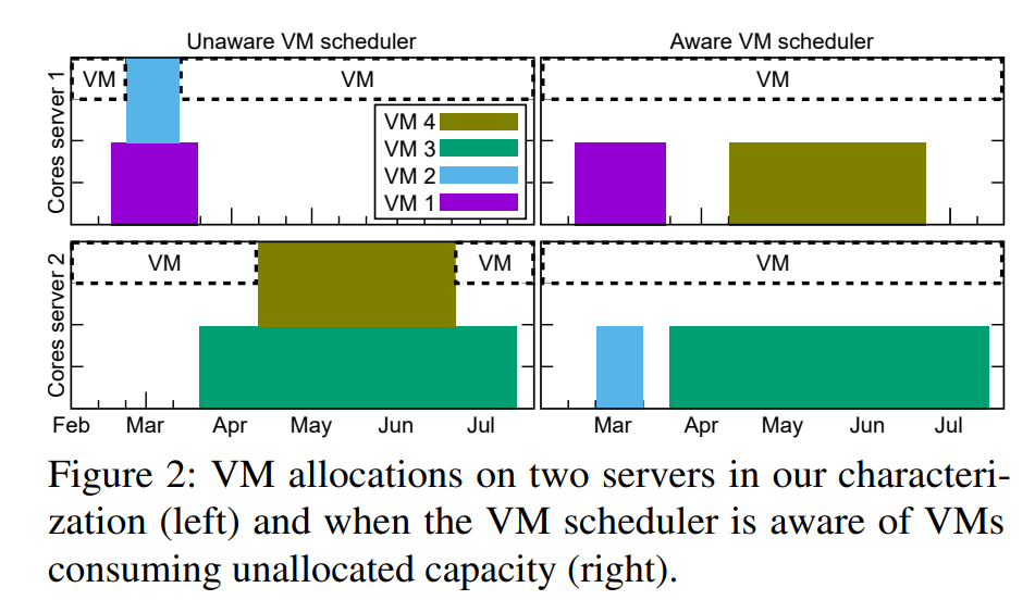
Cloud providers rent the resources they do not allocate as evictable virtual machines (VMs), like spot instances. In this paper, we first characterize the unallocated resources in Microsoft Azure, and show that they are plenty but may vary widely over time and across servers. Based on the characterization, we propose a new class of VM, called Harvest VM, to harvest and monetize the unallocated resources. A Harvest VM is more flexible and efficient than a spot instance, because it grows and shrinks according to the amount of unallocated resources at its underlying server; it is only evicted/killed when the provider needs its minimum set of resources. Next, we create models that predict the availability of the unallocated resources for Harvest VM deployments. Based on these predictions, we provide Service Level Objectives (SLOs) for the survival rate (e.g., 65% of the Harvest VMs will survive more than a week) and the average number of cores that can be harvested. Our short-term predictions have an average error under 2% and less than 6% for longer terms. We also extend a popular cluster scheduling framework to leverage the harvested resources. Using our SLOs and framework, we can offset the rare evictions with extra harvested cores and achieve the same computational power as regular-priority VMs, but at 91% lower cost. Finally, we outline lessons and results from running Harvest VMs and our framework in production.
Alok Kumbhare, Reza Azimi, Ioannis Manousakis, Anand Bonde, Felipe Frujeri, Nithish Mahalingam, Pulkit A. Misra, Seyyed Ahmad Javadi, Bianca Schroeder, Marcus Fontoura, and Ricardo Bianchini
in Proceedings of the USENIX Annual Technical Conference (ATC), 2021
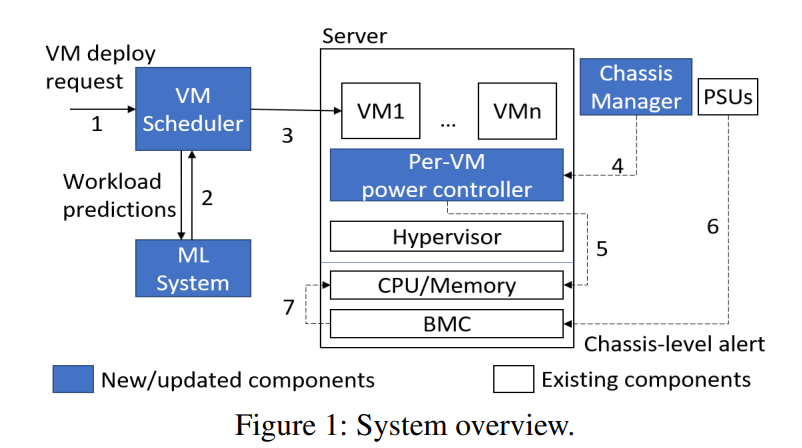
Datacenter designers rely on conservative estimates of IT equipment power draw to provision resources. This leaves resources underutilized and requires more datacenters to be built. Prior work has used power capping to shave the rare power peaks and add more servers to the datacenter, thereby oversubscribing its resources and lowering capital costs. This works well when the workloads and their server placements are known. Unfortunately, these factors are unknown in public clouds, forcing providers to limit the oversubscription so that performance is never impacted. In this paper, we argue that providers can use predictions of workload performance criticality and virtual machine (VM) resource utilization to increase oversubscription. This poses many challenges, such as identifying the performance-critical workloads from black-box VMs, creating support for criticality-aware power management, and increasing oversubscription while limiting the impact of capping. We address these challenges for the hardware and software infrastructures of Microsoft Azure. The results show that we enable a 2x increase in oversubscription with minimum impact to critical workloads.
Nofel Yaseen, Behnaz Arzani, Krishna Chintalapudi, Vaishnavi Ranganathan, Felipe Vieira Frujeri, Kevin Hsieh, Daniel S. Berger, Vincent Liu, Srikanth Kandula
in HotNets, 2021
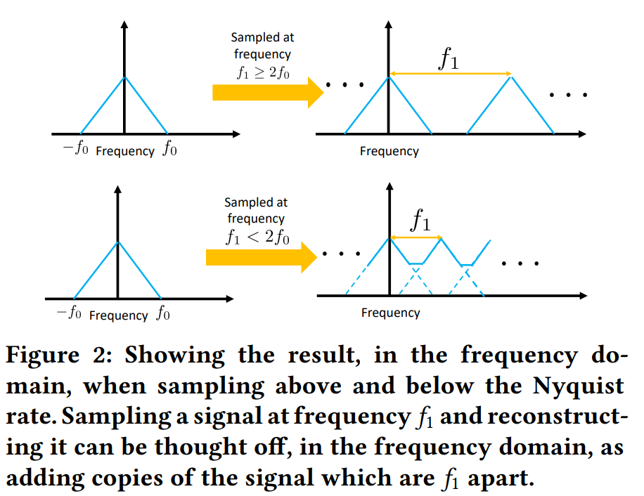
Continuously monitoring a wide variety of performance and fault metrics has become a crucial part of operating large-scale datacenter networks. In this work, we ask whether we can reduce the costs to monitor — in terms of collection, storage and analysis — by judiciously controlling how much and which measurements we collect. By positing that we can treat almost all measured signals as sampled time-series, we show that we can use signal processing techniques such as the Nyquist-Shannon theorem to avoid wasteful data collection. We show that large savings appear possible by analyzing tens of popular measurements from a production datacenter network. We also discuss the technical challenges that must be solved when applying these techniques in practice.
R Devon Hjelm, Bogdan Mazoure, Florian Golemo, Felipe Vieira Frujeri, Mihai Jalobeanu, Andrey Kolobov
in Preprint, 2022
 |  |  |
A broad challenge of research on generalization for sequential decision-making tasks in interactive environments is designing benchmarks that clearly landmark progress. While there has been notable headway, current benchmarks either do not provide suitable exposure nor intuitive control of the underlying factors, are not easy-to-implement, customizable, or extensible, or are computationally expensive to run. We built the Sandbox Environment for Generalizable Agent Research (SEGAR) with all of these things in mind. SEGAR improves the ease and accountability of generalization research in RL, as generalization objectives can be easy designed by specifying task distributions, which in turns allows the researcher to measure the nature of the generalization objective. We present an overview of SEGAR and how it contributes to these goals, as well as experiments that demonstrate a few types of research questions SEGAR can help answer.
Nolan Wagener, Andrey Kolobov, Felipe Vieira Frujeri, Ricky Loynd, Ching-An Cheng, Matthew Hausknecht
in NeurIPS, 2022
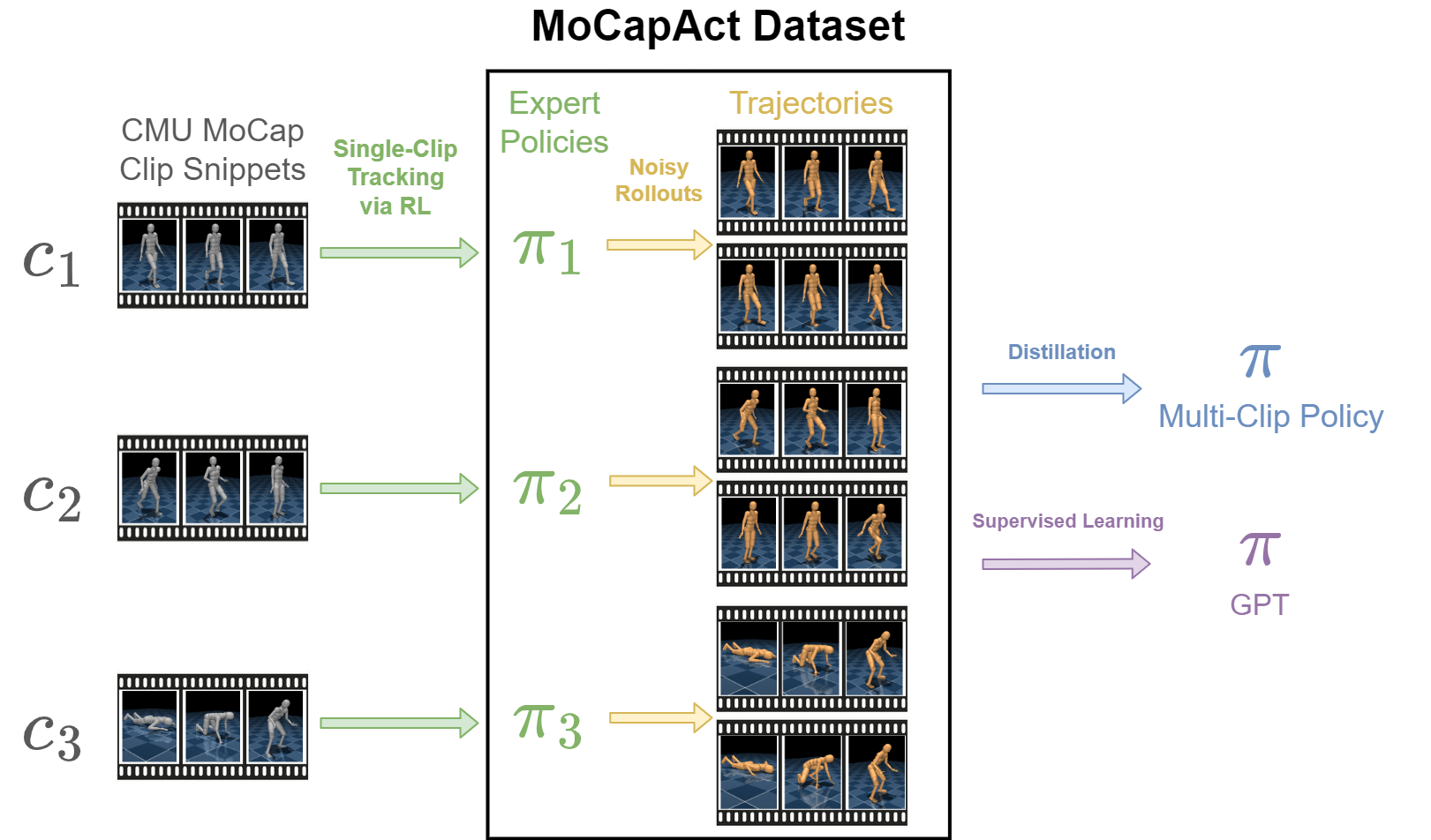
Control of simulated humanoid characters is a challenging benchmark for sequential decision-making methods, as it assesses a policy’s ability to drive an inherently unstable, discontinuous, and high-dimensional physical system. One widely studied approach is to utilize motion capture (MoCap) data to teach the humanoid agent low-level skills (e.g., standing, walking, and running) that can be used to generate high-level behaviors. However, even with MoCap data, controlling simulated humanoids remains very hard, as MoCap data offers only kinematic information. Finding physical control inputs to realize the demonstrated motions requires computationally intensive methods like reinforcement learning. Thus, despite the publicly available MoCap data, its utility has been limited to institutions with large-scale compute. In this work, we dramatically lower the barrier for productive research on this topic by training and releasing high-quality agents that can track over three hours of MoCap data for a simulated humanoid in the dm_control physics-based environment.
Shengpu Tang, Felipe Vieira Frujeri, Dipendra Misra, Alex Lamb, John Langford, Paul Mineiro, Sebastian Kochman
in Neurips Workshop, 2022
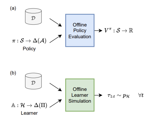
Modern decision-making systems, from robots to web recommendation engines, are expected to adapt: to user preferences, changing circumstances or even new tasks. Yet, it is still uncommon to deploy a dynamically learning agent (rather than a fixed policy) to a production system, as it’s perceived as unsafe. Using historical data to reason about learning algorithms, similar to offline policy evaluation (OPE) applied to fixed policies, could help practitioners evaluate and ultimately deploy such adaptive agents to production. In this work, we formalize offline learner simulation (OLS) for reinforcement learning (RL) and propose a novel evaluation protocol that measures both fidelity and efficiency of the simulation. For environments with complex high-dimensional observations, we propose a semi-parametric approach that leverages recent advances in latent state discovery in order to achieve accurate and efficient offline simulations. In preliminary experiments, we show the advantage of our approach compared to fully non-parametric baselines.
Yarin Perry, Felipe Vieira Frujeri, Chaim Hoch, Srikanth Kandula, Ishai Menache, Michael Schapira, Aviv Tamar
in NSDI (Best Paper Award), 2023
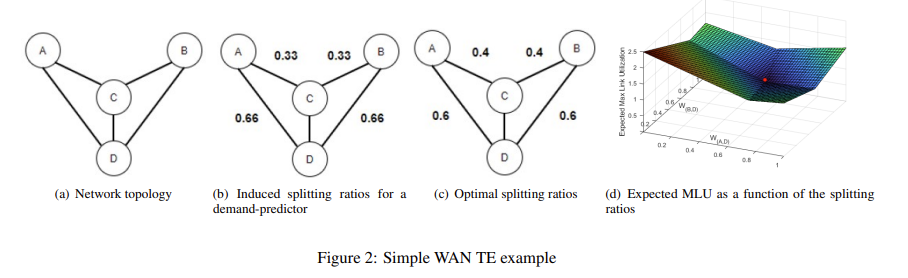
We explore a new design point for traffic engineering on wide-area networks (WANs): directly optimizing traffic flow on the WAN using only historical data about traffic demands. Doing so obviates the need to explicitly estimate, or predict, future demands. Our method, which utilizes stochastic optimization, provably converges to the global optimum in well-studied theoretical models. We employ deep learning to scale to large WANs and real-world traffic. Our extensive empirical evaluation on real-world traffic and network topologies establishes that our approach’s TE quality almost matches that of an (infeasible) omniscient oracle, outperforming previously proposed approaches, and also substantially lowers runtimes.
Banghua Zhu, Hiteshi Sharma, Felipe Vieira Frujeri, Shi Dong, Chenguang Zhu, Michael I. Jordan, Jiantao Jiao
in Preprint, 2023
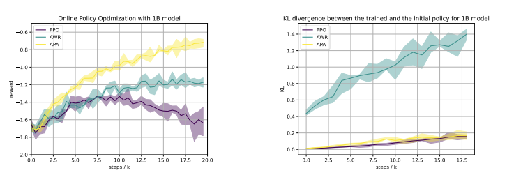
Reinforcement learning from human feedback (RLHF) has emerged as a reliable approach to aligning large language models (LLMs) to human preferences. Among the plethora of RLHF techniques, proximal policy optimization (PPO) is of the most widely used methods. Despite its popularity, however, PPO may suffer from mode collapse, instability, and poor sample efficiency. We show that these issues can be alleviated by a novel algorithm that we refer to as Advantage-Induced Policy Alignment (APA), which leverages a squared error loss function based on the estimated advantages. We demonstrate empirically that APA consistently outperforms PPO in language tasks by a large margin, when a separate reward model is employed as the evaluator. In addition, compared with PPO, APA offers a more stable form of control over the deviation from the model’s initial policy, ensuring that the model improves its performance without collapsing to deterministic output. In addition to empirical results, we also provide a theoretical justification supporting the design of our loss function.
Sean R. Sinclair, Felipe Frujeri, Ching-An Cheng, Luke Marshall, Hugo Barbalho, Jingling Li, Jennifer Neville, Ishai Menache, Adith Swaminathan
in International Conference in Machine Learning (ICML), 2023
Many resource management problems require sequential decision-making under uncertainty, where the only uncertainty affecting the decision outcomes are exogenous variables outside the control of the decision-maker. We model these problems as Exo-MDPs (Markov Decision Processes with Exogenous Inputs) and design a class of data-efficient algorithms for them termed Hindsight Learning (HL). Our HL algorithms achieve data efficiency by leveraging a key insight: having samples of the exogenous variables, past decisions can be revisited in hindsight to infer counterfactual consequences that can accelerate policy improvements. We compare HL against classic baselines in the multi-secretary and airline revenue management problems. We also scale our algorithms to a business-critical cloud resource management problem — allocating Virtual Machines (VMs) to physical machines, and simulate their performance with real datasets from a large public cloud provider. We find that HL algorithms outperform domain-specific heuristics, as well as state-of-the-art reinforcement learning methods.
Xin Wang*, Taein Kwon*, Mahdi Rad, Bowen Pan, Ishani Chakraborty, Sean Andrist, Dan Bohus, Ashley Fanello, Bugra Tekin, Felipe Vieira Frujeri, Neel Joshi, Marc Pollefeys
in International Conference on Computer Vision (ICCV), 2023

HoloAssist is a large-scale egocentric human interaction dataset, where two people collaboratively complete physical manipulation tasks. By augmenting the data with action and conversational annotations and observing the rich behaviors of various participants, we present key insights into how human assistants correct mistakes, intervene in the task completion procedure, and ground their instructions to the environment.
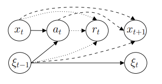
Rogerio Bonatti, Sai Vemprala, Shuang Ma, Felipe Frujeri, Shuhang Chen, Ashish Kapoor
in IROS, 2023
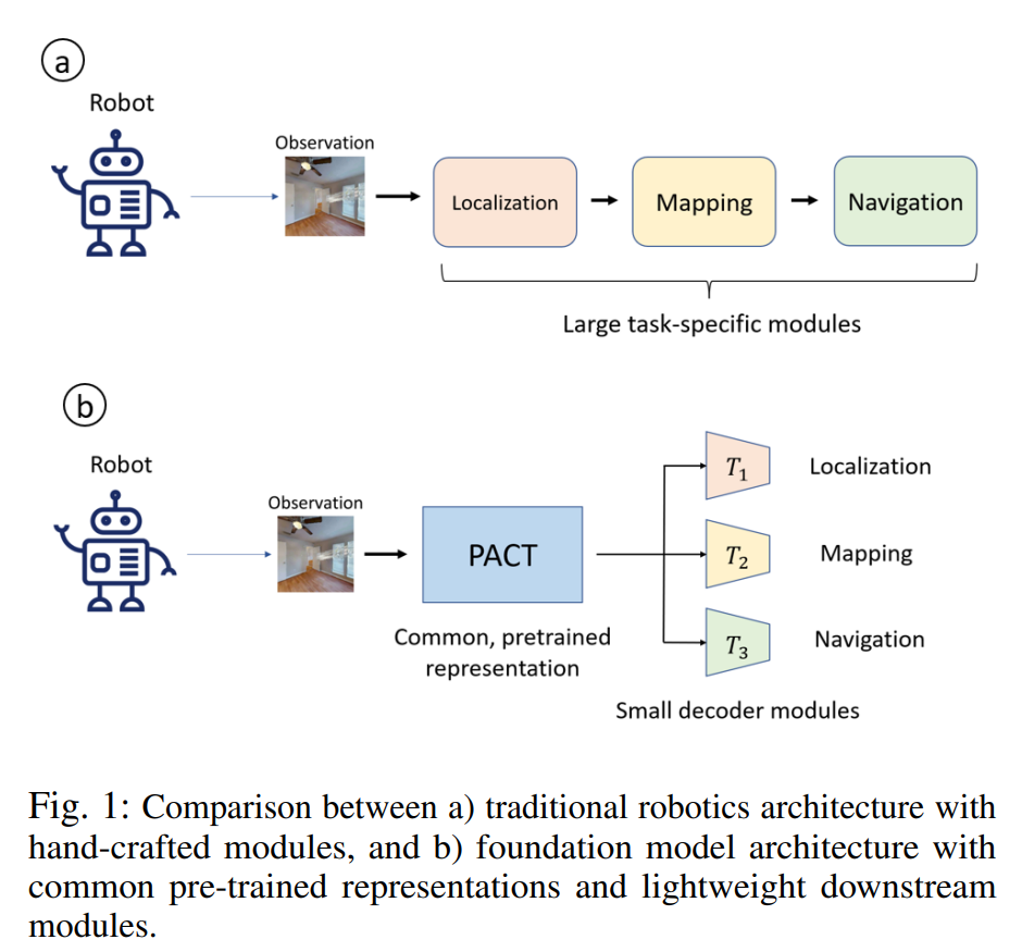
Robotics has long been a field riddled with complex systems architectures whose modules and connections, whether traditional or learning-based, require significant human expertise and prior knowledge. Inspired by large pre-trained language models, this work introduces a paradigm for pre-training a general purpose representation that can serve as a starting point for multiple tasks on a given robot. We present the Perception-Action Causal Transformer (PACT), a generative transformer-based architecture that aims to build representations directly from robot data in a self-supervised fashion. Through autoregressive prediction of states and actions over time, our model implicitly encodes dynamics and behaviors for a particular robot. Our experimental evaluation focuses on the domain of mobile agents, where we show that this robot-specific representation can function as a single starting point to achieve distinct tasks such as safe navigation, localization and mapping. We evaluate two form factors: a wheeled robot that uses a LiDAR sensor as perception input (MuSHR), and a simulated agent that uses first-person RGB images (Habitat). We show that finetuning small task-specific networks on top of the larger pretrained model results in significantly better performance compared to training a single model from scratch for all tasks simultaneously, and comparable performance to training a separate large model for each task independently. By sharing a common good-quality representation across tasks we can lower overall model capacity and speed up the real-time deployment of such systems.
Garrett Thomas, Ching-An Cheng, Ricky Loynd, Felipe Vieira Frujeri, Vibhav Vineet, Mihai Jalobeanu, Andrey Kolobov
in CoRL, 2023

A rich representation is key to general robotic manipulation, but existing model architectures require a lot of data to learn it. Unfortunately, ideal robotic manipulation training data, which comes in the form of expert visuomotor demonstrations for a variety of annotated tasks, is scarce. In this work we propose PLEX, a transformer-based architecture that learns from task-agnostic visuomotor trajectories accompanied by a much larger amount of task-conditioned object manipulation videos — a type of robotics-relevant data available in quantity. The key insight behind PLEX is that the trajectories with observations and actions help induce a latent feature space and train a robot to execute task-agnostic manipulation routines, while a diverse set of video-only demonstrations can efficiently teach the robot how to plan in this feature space for a wide variety of tasks. In contrast to most works on robotic manipulation pretraining, PLEX learns a generalizable sensorimotor multi-task policy, not just an observational representation. We also show that using relative positional encoding in PLEX’s transformers further increases its data efficiency when learning from human-collected demonstrations. Experiments showcase PLEX’s generalization on Meta-World-v2 benchmark and establish state-of-the-art performance in challenging Robosuite environments.
Felipe Vieira Frujeri*, Ida Momennejad*, Hosein Hasanbeig*, Hiteshi Sharma, Robert Ness, Nebojsa Jojic, Hamid Palangi, Jonathan Larson
in NeurIPS, 2023

We propose CogEval, a cognitive science-inspired protocol for the systematic evaluation of cognitive capacities in Large Language Models. The CogEval protocol can be followed for the evaluation of various abilities. And systematically evaluate cognitive maps and planning ability across eight LLMs. We base our task prompts on human experiments, which offer both established construct validity for evaluating planning, and are absent from LLM training sets. We find that, while LLMs show apparent competence in a few planning tasks with simpler structures, systematic evaluation reveals striking failure modes in planning tasks, including hallucinations of invalid trajectories and falling in loops.
Published:
This is a description of your talk, which is a markdown files that can be all markdown-ified like any other post. Yay markdown!
Published:
This is a description of your tutorial, note the different field in type. This is a markdown files that can be all markdown-ified like any other post. Yay markdown!
Published:
This is a description of your talk, which is a markdown files that can be all markdown-ified like any other post. Yay markdown!
Published:
This is a description of your conference proceedings talk, note the different field in type. You can put anything in this field.
Undergraduate course, University 1, Department, 2014
This is a description of a teaching experience. You can use markdown like any other post.
Workshop, University 1, Department, 2015
This is a description of a teaching experience. You can use markdown like any other post.